

Header image: Moderate cross-country slopes (Photo: By Erik W. Kolstad – Flickr, CC BY 2.0,)
Here’s a particular genre of article that relies on multiple data collection sites, such as studies analyzing cross-country or cross-county data:
It has been well established that X affects Y. However, the magnitude of the effects plausibly depends on some context factor Z. In the following cross-country analysis, we show how the role of X for Y varies depending on Z. This is usually followed by, in the best case, some variation of a multilevel regression analysis that regresses Y onto X, Z, and their interaction (potentially with additional controls). [1]In worse cases, it is followed by some bespoke multi-step procedure in which, for example, researchers first calculate some country-level group differences and then correlate these with Z. All of the following points still apply to these scenarios, plus they also have some additional issues that we are going to ignore here because the best case scenario is already problematic enough.
X, Y, and Z vary by literature; some examples:
- X: gender, Y: pursuit of a STEM degree, Z: the country-level Global Gender Gap Index (GGGI). Voilà, we end up with the so-called gender-equality paradox that claims that gender differences are larger in more gender-equal countries even though one may naively assume that gender equality reduces gender differences.
- X: income, Y: generosity in the so-called dictator game, Z: state-level income inequality. Voilà, only under conditions of high inequality does income foster a sense of entitlement with a corresponding decrease in generosity.
- X: resource-acquisition abilities (level of education, income), Y: attention one’s online dating profile receives, Z: the country-level sex ratio. Voilà, cross-cultural variance in the role of resource-acquisition ability is sensitive to local competition.
In the following, I want to discuss some concerns that commonly apply to articles from this genre. I’m going to assume throughout that the intended claim is that “Z affects the magnitude of the effect of X on Y,” because that’s usually the story being told (with more or less strategic ambiguity/clarity about estimands/vague gesturing towards theory testing). I am not going to discuss the “ecological fallacy,” because while this is what people usually bring up when these types of studies are discussed, I’m profoundly confused about what they actually mean by it.[2]It seems to be used for a hodgepodge of concerns that mostly have in common that they do apply to these types of studies.
Instead, I’m going to discuss the following:
Level 1: The causal identification of the effects of X on Y
Level 2: The causal identification of the effect of Z on the effects of X on Y
Level 2: Non-standard confounding factors to consider
Followed by suggestions for how to improve moderated cross-country regressions.
Level 1: The causal identification of the effects of X on Y
This doesn’t have anything to do with the cross-country part yet, so you might skip this section if you are already aware that you are going to need an identification strategy to estimate the causal effect of X on Y for the whole cross-country thing to become coherent. I’m still including this here because while everybody seems aware that correlation does not imply causation, somehow that tends to be forgotten once the research question gets more complex.
One identification strategy could be to actually conduct an experiment and randomly assign different levels of X, which would be a heavily design-based solution. Another identification strategy could be to figure out the relevant confounders and adjust for them in the appropriate manner, which would be more of a model-based solution.[3]That is more likely to raise eyebrows in certain fields because of the strong assumption it relies on, but that doesn’t mean it’s impossible in principle. See this primer I wrote for an introduction to the logic of this approach. And then there’s stuff in between, like natural experiments. For example, if you’re interested in the gender-equality paradox, you may rely on the assumption that biological sex is assigned pretty much randomly at birth, which would mean that you can interpret associations with biological sex as causal effects of sex, under some additional assumptions.[4]For example, inclusion in the sample shouldn’t be affected by sex – if you find associations with biological sex among psychology students, but being a woman strongly affects the probability of studying psychology, as do other factors, then you cannot interpret these causally. That’s because inclusion in the sample is a collider (sex → sample inclusion ← other stuff) that is conditioned on (the variable is TRUE for everybody in your data). Schuessler and Selb (2023) have a nice introduction to reasoning about these scenarios with causal graphs. One specific situation in which this can get tricky is looking at very old people – you can usually not include the dead in your sample, and men tend to die earlier, so at high ages the remaining men went through a slightly different survival filter than the remaining women.
What if you don’t have a proper identification strategy for X → Y but carry on regardless? Essentially, your analysis will look at how Z is associated with some (conditional or unconditional, depending on what else is in the model) association between X and Y. The magnitude of an association may vary for all sorts of reasons that have nothing to do with the effects of interest.
For example, the magnitude of some non-causal part of the association may vary depending on the strength of Z, because Z affects some confounding path. It is admittedly hard to intuitively come up with such “modification of the strength of confounding”, but that doesn’t mean it’s implausible – it’s just that we don’t often think about these things. For example, consider the idea that income inequality moderates the effect of income on generosity. Age may affect both income and generosity; and the effect of age on income may be stronger in more unequal countries.
In any case, a failure of imagination is not a very good identification strategy, even if some people like to pretend otherwise. If all else fails, just list all major confounders between X and Y that you can come up with and consider whether it’s plausible that some country-level variable affects how strongly those confounders affect your X or Y. It usually is; there’s no reason why “Z affects this effect of interest” should generally be more plausible than “Z affects this other effect which confounds the thing I’m interested in.” The universe just isn’t kind like that.
The cross-country part
Level 2: Small sample sizes
Let’s start with something straightforward. If your higher-level units are literally countries, well, there are only so many countries in the world. To be more precise, there are exactly 200ish, according to what I consider the authoritative source on the matter. If you pick some smaller geographical unit,[5]or if you sample countries repeatedly over time – something to which we will return later you may end up with a larger population, but don’t forget that for sample size, you actually need to sample those units. So, usually, the sample size on the second level will be rather small.
What does that mean for your analysis? Thinking in terms of multi-step approaches helps hone the right intuitions here, even if they’re not necessarily the best analysis you can pull off. In the first step, you estimate the causal effect per country (or per geographical unit). If you have a lot of people in a country, that estimate will be more precise; if you have fewer people, that estimate will be less precise. But let’s imagine the best-case scenario in which you have a humongous per-country sample, so that the estimate is so precise that you can just assume it’s pretty much on point. In the next step, you take those per-country effect estimates and correlate them with Z across countries. Even if your per-country effects are estimated with perfect reliability, you end up with a correlation across as many observations as you have countries in your data. And if you usually wouldn’t consider a correlation across 30 people particularly trustworthy (for example, because you know that correlations bounce around a lot in small samples), you shouldn’t consider a correlation across 30 countries particularly trustworthy either.
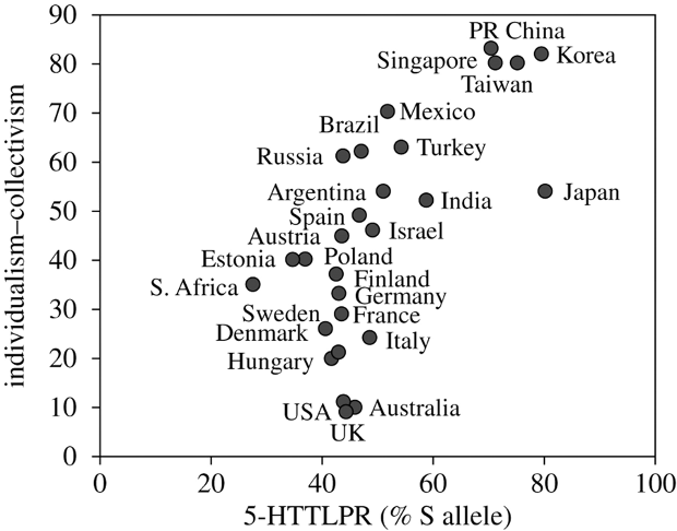
Correlation between Hofstede’s individualism-collectivism index (reverse-scored) and frequency of S allele carriers of the 5-HTTLPR across 29 nations, r(29) = 0.70, p < .0001. From Chiao and Blizinsky (2009), Creative Commons Attribution License. Courtesy of Moin Syed.
It is, of course, a lot harder to sample individuals from 30 countries than it is to sample 30 individuals. Unfortunately the standard errors in your estimates don’t care about that; once again, the universe is just unfair like that. Given how hard it is to collect good cross-country data, one may think it should be rewarded with a publication even if the resulting evidence is weak – I, unlike the universe, am highly sympathetic to that idea as long as the conclusions in the manuscript are appropriately calibrated to the strength of the evidence – but this is an entirely different argument to have. So let’s go back to the stats.
In fact, the small sample size issue will often loom larger than it appears upon first glance, because all the additional Level 2 causal inference concerns mean that you don’t just want to correlate Z with the effects across countries; you want to do something more complex.
The causal identification of the effect of Z on the effects of X on Y
If you want to find out whether country-level Z affects the effects of X on Y, you will need some sort of causal identification strategy. This may come as a surprise because, at least in psychology, most people do not clearly distinguish between “Z is associated with the magnitude of the effects of X on Y” and “Z causally affects the magnitude of the effects of X on Y.” But this distinction is quite fundamental; it’s essentially the difference between correlation and causation, except that one of the variables is “the magnitude of the effects of X on Y.” To be fair, psychologists’ understanding is not exactly aided by the fact that the terminology for this distinction is inconsistent across and within fields; Ruben and I provide a small collection of different terms in our 2021 paper on interactions, which has a dedicated section on the causal identification of interactions.
To make the issue more specific, imagine that you found that the magnitude of the effects of wearing red dresses on how attractive women are rated is positively associated with gender equality. Now, how do you know this is a story about gender equality as opposed to, let’s say, a story about GDP per capita? After all, many of the countries that score high on gender equality metrics also happen to be quite wealthy nations in the global North, so there’s that. Or maybe the red dress effect is about urbanization? Education? Religiosity? Democracy? The welfare state? Individualism? Fertility rates? Instagram penetration? The size of the agricultural sector? All of these things are likely correlated on the country-level, so all of them are potential alternative explanations. The key inferential problem is that an association between gender equality and the size of the red-dress effect does not show that gender equality causally changes the red-dress effect. Rather, gender equality may merely mark a broader bundle of country-level differences.
Now, of course, things in this bundle aren’t perfectly correlated, so under the assumption that they are potential confounders[6]And not mediators or colliders, because statistical control requires causal justification. How to figure out which is which on the country level? Honestly, I’m not sure. of the effect of interest (Z → Magnitude of the effects of X on Y), we can try to account for them in our analysis by (1) including the alternative country-level explanations as predictors and (2) including the interaction between the alternative country-level explanation and the X of interest. The second part is easy to forget, but interaction effects need interaction controls – the alternative explanation is not that GDP affects how attractive women are rated; the alternative explanation is that GDP affects the extent to which red dresses affect attractiveness ratings. So, you need that interaction control to rule out GDP is bamboozling you.
But, wait a second – aren’t there a ton of potential country-level confounders that would need to be included, including their interactions? And didn’t we just say that the sample sizes on this level are usually small? If you combine these two facts, it may look like this endeavor is futile; you’re going to run out of statistical power immediately. That is indeed often going to be the case. You don’t want your results to be badly confounded, so not controlling is not an option; once you do control, you may end up with the conclusion that you can’t conclude anything. To be entirely clear, that would be the correct conclusion. It’s just not a fun one.[7]Bloody universe, amirite?
Well, it’s bad, getting worse: “Non-standard” confounding factors to consider
If I hated to be the bearer of bad news, I wouldn’t have specialized in research methods.[8]To make this news more palatable, you can pretend I wrote these lines wearing a red dress.
In the context of moderated cross-country regressions, there are lots of things that can mess things up on Level 2 that aren’t the usual “vanilla” confounders. Countries share history and culture that lead to additional confounding across space (and time, for that matter), a point that has been made for the gender-equality paradox by Berggren and Bergh (2025). The Protestant West in particular may just be built different. On the one hand, gender stereotypes (as we usually understand and measure them) may be more differentiated there; on the other hand, this region tends to be quite rich and developed with corresponding low numbers on indicators of country-level gender inequality. Looking at the association between gender gaps and country-level inequality within that cultural cluster, not much of a gender-equality paradox can be found according to the authors. So maybe the whole thing is not about gender equality, but rather about Protestants being weird.
Relatedly, considering measurement, if you’re going to compare effects across countries, you’ll have to worry about all sorts of concerns of measurement invariance. For example, sometimes translated questionnaires are not very sensible or even just simply really bad. And then a measure may mean something different in a different country altogether. Berggren and Bergh discuss this for the case of gender gaps in chess participation: Western countries have a long cultural tradition of men playing it, and therefore also reasonably stronger gender stereotypes associated with it; in other places such a stereotype needn’t even exist and so gender differences in chess participation don’t have much to do with stereotypical gender behavior in the first place. For another example, consider soccer aka association football aka just football, which is definitely more female-coded in the US than it has been traditionally in most of the rest of the world.
You can also get scaling issues when countries differ in the level of the outcome. For example, maybe in some countries women are generally rated as more attractive. At some point you get close to the ceiling of the scale, which means that in those countries, it will be hard to detect any additional positive effect of any possible treatment. Maybe you are interested in how wearing red affects attractiveness ratings cross-culturally but in some places women are already mostly rated 10/10 to begin with. In those places, it will necessarily look like wearing red makes little difference simply because the scale stops. This can lead to “spurious moderation” (Box 1 of our interactions paper), which should be addressed by more appropriate statistical modeling, rather than by speculation about how the regional prevalence of juicy berries modifies the visual salience of sexy red dresses.
And of course, you can get scaling issues if people in different countries use the scale in a different manner; that’s essentially a given.[9]Looking at you, Finland, “happiest” country in the world.
In general, differential data quality is a big one. I occasionally see research that relies on completely different sampling strategies per country. That may be reasonable for pragmatic reasons; but it’s kinda hard to say what exactly can be learned if an effect differs between (1) an undergraduate student sample from a highly gender-equality country, (2) an online opt-in panel from a medium gender-equality country, and (3) a sample from that one village one of the investigators happened to visit during their PhD studies in a low gender-equality country. One can try to take these differences into account appropriately (see, e.g., Deffner et al., 2022), but it should come as no surprise that this means stacking assumptions on top of assumptions. Also, as far as I can tell, barely anybody does that in practice.[10]Which I totally get. Dominik Deffner had to write Stan code for our paper on cross-cultural generalizability. I wouldn’t want to do that either.
Of course, our country-level measure Z could also have all sorts of issues, and these will hit harder if only a small number of countries are included. For example, GDP per capita has received a lot of flak for a variety of reasons.[11]Part of it is the question of what counts into it and what doesn’t; part of it how reliable and comparable our data on those things that count are; another part is whether simply dividing by population size is really good enough (e.g., Kratochvíl & Havlíček, 2024). And there are probably other reasons as well, apparently people love to hate on GDP per capita. In general, I have the impression that psychological researchers think of economic indices as hard indicators without the usual measurement issues; Works in Progress has an excellent article titled “Where inflation comes from” to disabuse anyone from such notions. Considering country-level cultural variables, Moin Syed was so kind to provide various sources. And considering country-level health information, following Saloni Dattani’s work has disabused me of the notion that we know much at all, which is a shame. Death and taxes may be certain, but we’re quite uncertain about how many people are affected by death, let alone what they are dying of. I’m just assuming the tax data situation isn’t that much better.
But at some point, talking about problems stops being fun, even for a research methods person.

Ways to improve moderated cross-country regressions
Despite the title of this post, I still think there are things friends can do to improve their friends’ moderated cross-country regressions, at least somewhat.
Better identification strategies for Z
One obvious contender is looking for a better identification strategy for the effect of the country-level variable Z. Unless you have international leverage way beyond the wildest conspiracy theories, randomizing Z across countries is probably out of the question. Maybe for some Z there could be viable surrogate experiments in which something is randomized to mimic the effects of a low Z or high Z environment, but just given what these experiments traditionally look like in psychology, color me skeptical.

But there are things in between third-variable adjustment and full-blown randomization that may allow for more plausible inferences. Broadly speaking, this makes us end up somewhere in the realm of natural experiments, where we hope for some naturally occurring variation that is more plausibly not quite as hopelessly confounded. For example, there could be adjacent regions that are highly similar in many respects, except for some historic circumstance that affects Z. Comparing those to draw conclusions about the effect of Z still requires assumptions which can be wrong, but it’s better than pretending that countries are completely independent entities that literally only vary with respect to Z.
Alternatively, one may want to look at associations within country, over time. If gender equality impacts gender differences, then one would expect gender differences to (slowly) change as gender equality changes over time. Now this isn’t foolproof either, but associations within countries are not confounded by time-invariant country-level confounding (that is, the stable stuff that makes countries different from each other in a consistent manner over time). So hey, that’s one less class of confounders to worry about! The logic here is very much the same as for within-person analyses – looking within countries isn’t inherently necessary to identify the causal effects, it also most definitely isn’t sufficient (because of time-varying confounding), but it can help quite a bit. Just make sure your analyses are actually within-country.[12]Random intercepts in a multilevel model are not enough; you need fixed effects/a Mundlak device/some mean-centering to do the trick.
More transparency
Generally, when reading papers with moderated cross-country regressions, I tend to be frustrated by the lack of transparency. It’s one thing to conduct an analysis that rests on questionable assumptions, it’s another thing to not even show what goes into it. Sometimes, readers literally only get the regression coefficient for the interaction term (p < .05), as if that was all there is to the data.
But there’s so much other stuff that I would be interested in, and that would be genuinely helpful to evaluate the credibility of the whole story.
For example, if the analyses plausibly identify the effects of X on Y, I would very much want to see the model-implied average effect for each of the included countries. Now, depending on how you set up the model, these may be hidden somewhere in some random slopes and not that easy to get out. But that isn’t really a good excuse in 2026. When in doubt, marginaleffects.
Likewise, I want to see how the included countries score on Z. For some reason, this is routinely done for one type of study (where people are interested in regional differences and apparently like to show off pretty maps) but not for another one (where people just want those differences to moderate something). There are different ways to achieve this, one being a pretty map.
Another one is showing a scatterplot of Z against the estimated effect of X on Y, with the individual data points actually labelled – that is, actually telling people which country is which. Again, this can be somewhat fiddly, but it is tremendously helpful to (1) evaluate whether Z seems to reasonably match what we know about the countries at hand and to (2) visually evaluate alternative explanations. Maybe all the results are driven by the Nordic countries just being built differently? Maybe it’s a group of countries of which we know that they are quite distinct on some third factor? Maybe it’s just Japan?
As always, this type of transparency can be self-defeating. It’s no good presenting the whole picture when the whole picture is just going to raise eyebrows, as long as you can still get through by hiding a lot. From that angle, I think the best thing we can do as a field, collectively, is to raise our standards for this type of research. If you’re a reviewer, say something and demand more transparency. Urge the authors to discuss alternative explanations. Don’t let yourself be lulled by soothing storytelling.
In the end, the types of claims that are usually intended when researchers conduct naive moderated cross-country regressions are just very hard to establish in a credible manner. These are sweeping narratives about why the world looks the way it does, across space and often also across time. Expecting a haphazard regression analysis based on cross-national data (that often happens to be somewhat conveniently already available) to provide good evidence for such a narrative is maybe asking a bit too much, in particular when you add the usual psych issues (messy measurement, unobservable outcomes, and even causes, which may as well be non-manipulable).
So what would I recommend if a friend actually wanted to run a moderated cross-country regression? I’d probably suggest they spend their time on something more fruitful, unless they’re absolutely sure what they are doing there.[13]I trust my friends to be well-calibrated on that matter but YMMV. Or, alternatively, they may turn their work into an educational piece on why that type of analysis is so doomed. My enemies, on the other hand, I let add random slopes for continents, and throw in some Hofstede dimensions and call them robustness checks.
Footnotes
| ↑1 | In worse cases, it is followed by some bespoke multi-step procedure in which, for example, researchers first calculate some country-level group differences and then correlate these with Z. All of the following points still apply to these scenarios, plus they also have some additional issues that we are going to ignore here because the best case scenario is already problematic enough. |
|---|---|
| ↑2 | It seems to be used for a hodgepodge of concerns that mostly have in common that they do apply to these types of studies. |
| ↑3 | That is more likely to raise eyebrows in certain fields because of the strong assumption it relies on, but that doesn’t mean it’s impossible in principle. See this primer I wrote for an introduction to the logic of this approach. |
| ↑4 | For example, inclusion in the sample shouldn’t be affected by sex – if you find associations with biological sex among psychology students, but being a woman strongly affects the probability of studying psychology, as do other factors, then you cannot interpret these causally. That’s because inclusion in the sample is a collider (sex → sample inclusion ← other stuff) that is conditioned on (the variable is TRUE for everybody in your data). Schuessler and Selb (2023) have a nice introduction to reasoning about these scenarios with causal graphs. One specific situation in which this can get tricky is looking at very old people – you can usually not include the dead in your sample, and men tend to die earlier, so at high ages the remaining men went through a slightly different survival filter than the remaining women. |
| ↑5 | or if you sample countries repeatedly over time – something to which we will return later |
| ↑6 | And not mediators or colliders, because statistical control requires causal justification. How to figure out which is which on the country level? Honestly, I’m not sure. |
| ↑7 | Bloody universe, amirite? |
| ↑8 | To make this news more palatable, you can pretend I wrote these lines wearing a red dress. |
| ↑9 | Looking at you, Finland, “happiest” country in the world. |
| ↑10 | Which I totally get. Dominik Deffner had to write Stan code for our paper on cross-cultural generalizability. I wouldn’t want to do that either. |
| ↑11 | Part of it is the question of what counts into it and what doesn’t; part of it how reliable and comparable our data on those things that count are; another part is whether simply dividing by population size is really good enough (e.g., Kratochvíl & Havlíček, 2024). And there are probably other reasons as well, apparently people love to hate on GDP per capita. |
| ↑12 | Random intercepts in a multilevel model are not enough; you need fixed effects/a Mundlak device/some mean-centering to do the trick. |
| ↑13 | I trust my friends to be well-calibrated on that matter but YMMV. |
I love all the causal posts, and this one no less than the others!
I was trying to imagine some DAGs throughout, even if they are usually less intuitive when discussing interactions. In the level 1 example, I think it’s a fair attempt to represent “modification of the strength of confounding” by having Z mediate (partly or fully) either effect of confound U on X or Y.
In general though, things aren’t always easy for me, since we can’t have arrows pointing at other arrows. I think one should start from the assumption that if two variables affect something, so does their interaction, right?
Thank you 🙂 Yes, the DAGs are not that helpful for depicting/reasoning about interactions (although people have suggested all sorts of modifications to make them more explicit). But yes, in the DAG-logic, when multiple variables affect another jointly, they may always interact, so that could be taken as the default assumption (and assuming that interaction away would be an intentional decision). X –> Y, X <-- U --> Y, Z –> Y (or X) would be sufficient to depict a scenario in which Z modifies the strength of confounding.