Testing for measurement invariance is one of those things where researchers roughly fall into two categories. Either they consider it an incomprehensible and arcane practice that only nerds could ever care about (probably the majority), or they consider it an indispensable and mandatory step before any sort of group comparison (nerds!). In any case, it is treated mostly as a statistical ritual, either an exotic or a mundane one.[1]A possible exception to this may be the literature on intelligence, in which measurement invariance is a relevant topic of substantive debate.
Measurement invariance is usually defined as a statistical property that shows that a measure (e.g., an ability test, or a personality questionnaire) measures the same construct in different groups (e.g., in North Americans and South Africans; in young people and old people). Another way to put it is that the measure works the same way in each group. In either case, when a measure is invariant, we can use it to compare the construct between the groups (e.g., to test whether there are personality differences between young people and old people). Or so they say.[2]John Protzko told me he received pushback for saying that people say measurement invariance implies that the measure measures the same thing in different groups. So, in his preprint on measurement invariance, he now reviews the evidence that measurement invariance is commonly interpreted this way–which it is.
This always sounded like magic to me. I’m sometimes uncertain whether a given measure measures anything at all – how could a statistical procedure be so much smarter and determine whether the same potentially ineffable thing is being measured in different groups, just based on some correlations and mean values? It just strains credulity.
In the following, I will provide a brief conceptual introduction to measurement invariance, but I will also try to convince you of two things. First, bad news: tests of measurement invariance indeed cannot achieve magical things. Second, good news: measurement invariance is much more interesting than the literature pretends. Measurement invariance often appears like a mandatory statistical bar that needs to be cleared before interesting substantive statements can be made. This mindset renders a lack of invariance (i.e., variance) a tragedy to be avoided at all cost because it puts a premature end to a substantive project. But in fact, it is a lack of measurement invariance that tells us there may be something substantively interesting going on. As always, the secret ingredient will be a causal perspective.
Four Levels Total Invariance
Level 1, configural invariance: All your item are belong to us
Configural invariance means that the “form” of the models is the same in the groups of interest. Form entails both the number of latent variables and whether the loadings are non-zero to begin with. For example, let’s say we were interested in whether an extraversion measure consisting of five items is “configurally invariant” for young and old people (Fig. 1). What we would do to check this is run a one-dimensional factor model in the young group, and another one in the old group. If the one-dimensional model fits in both groups, and no item belongs to the construct in one group but not the other one, we could claim configural invariance. Or, more correctly, we could not reject the hypothesis of configural invariance.
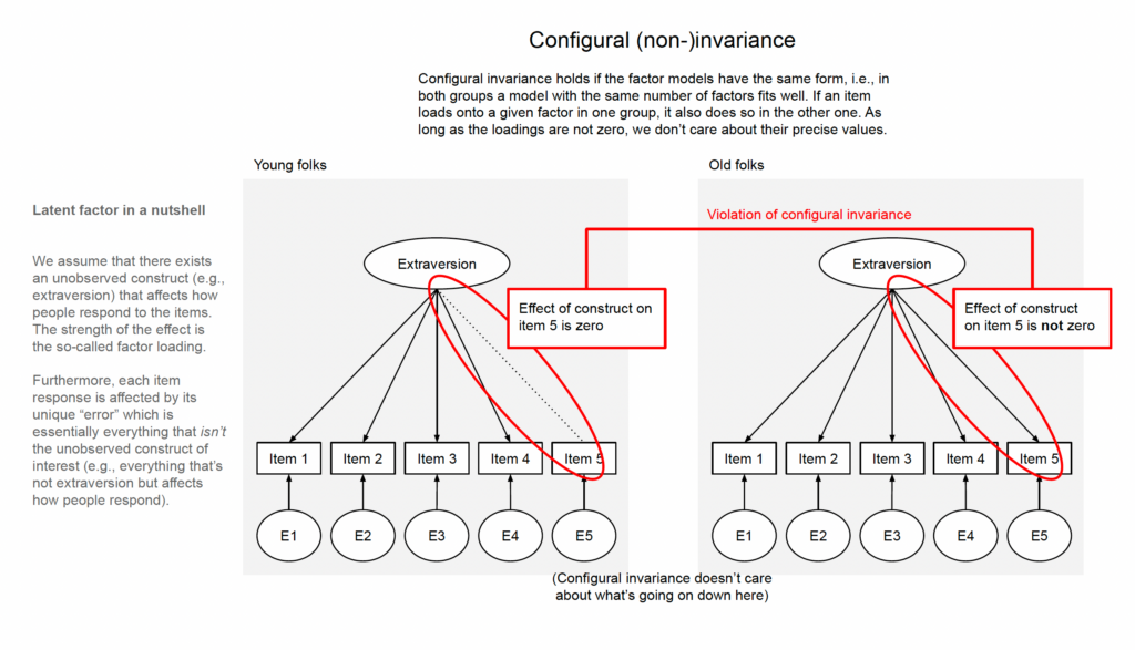
Configural invariance is mostly like a weaker form of metric invariance, which is why we are going to discuss the interesting substantive stuff in the next section.
Level 2, metric invariance: Things are getting loaded
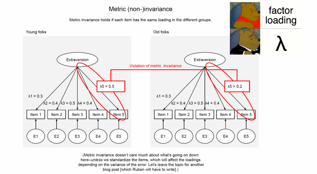
Metric invariance means that for each item, the loading of the factor on the item is the same in the two groups (or, again more precisely, that we cannot reject the hypothesis that the loadings are the same), see Fig. 2. So, for example, the loading of extraversion on “I am the life of the party” needs to be the same for young people as for old people. The standard way to test this is to run a multi-group structural equation model (SEM) and then constrain the loadings to be equal across groups and check how the model fit changes; if it gets a lot worse, we would reject the equality of loadings and thus reject metric invariance.[3]A little bit worse may be okay. Always check with your local statistician or the literature if you have any concerns about debates about the appropriate cut-offs for measurement invariance testing.
What does that mean, though? Let’s take a step back. In structural equation modeling, we are trying to explain the data through a model. The data are our observed item responses; in particular the associations between them.[4]More technically, the data that are being explained in structural equation models are usually the elements of the variance-covariance matrix (a matrix that for each item contains its variance and its covariance with all other items; think correlation matrix but in unstandardized). Thus, SEM results can often be fully reproduced from the variance-covariance matrix alone. Sometimes, the mean structure is also modeled (e.g., when testing scalar invariance, see later section). The model is a latent variable model in which some (unobservable) construct affects the item responses, and the magnitude of these causal effects is quantified by the corresponding loadings. So, this is a causal model. Measurement invariance means that the same causal model can explain the data in all groups.
Before we get to the galaxy-brain interpretation of this, let’s talk about a corollary: when we are testing for measurement invariance, we are testing causal models based on observational data. Any factor model is a causal model based on observational data. Oops-a-daisy! The results are always conditional on causal assumptions; here, the assumed factor model. Without those assumptions, we don’t get anywhere because the observed associations between the items could be explained by an infinitude of alternative data-generating mechanisms.[5]Here I am subscribing to a realist interpretation of factor models, in which the arrows are arrows and not a shorthand for “an association but somehow also directed.” The realist stance is forwarded in older writings by Borsboom, Mellenbergh and van Heerden (2003, 2004). A lot of researchers are probably more comfortable subscribing to a pragmatist interpretation in which a factor model is just a good way of summarizing a large number of items. I am not sure such an interpretation is 100% consistent. First of all, when calculating a factor score, items with higher loadings will have a bigger impact. Statistically speaking, those will be the items that have higher correlations with other variables. But why would we want to give higher weight to those items when the goal is to simply summarize the variables? Giving equal weights to the items (aka, just taking the average) seems more justifiable if we are completely agnostic to what caused the data (and thus also about how error may have affected values). Second, once we try to do anything else with those latent variables, inferences can end up badly biased if the true data generating mechanism was a different one (Rhemtulla et al., 2020). Unless somebody convinces me otherwise (come at me pragmabro), I think the pragmatist interpretation is mostly a cope to avoid facing that much of empirical psychology rests on very strong assumptions. That puts “I’m just using this factor model for pragmatic reasons” into the same category as “oh no I do not want to make causal claims I am just trying to do prediction” (see footnote 12) and “non-causal mediation analysis” (which isn’t a thing; mediation is statistically indistinguishable from confounding–the difference lies in causal assumptions).
So saying that measurement invariance establishes that the same thing is measured in different groups is a bit of a stretch. It’s more that measurement invariance tests whether certain things are the same across groups, conditional on the assumptions that the latent variable model holds.
But let’s get to the galaxy-brain take, which was once revealed to me in a dream manuscript by Denny Borsboom.[6]And then shortly afterwards I stumbled across it again in Paulewicz and Blaut’s paper on the general causal cumulative model of ordinal response. Baader-Meinhof much Measurement invariance implies that all effects of the group variable on the items are fully mediated by the latent construct.[7]More generally speaking (and still keeping things casual), measurement invariance implies that all group differences in the items “go through” the latent construct. So, measurement invariance would also be violated if there is a common cause that confounds the group variable with the items. In such a scenario, the measure would be non-invariant, but it is a type of non-invariance that can be “explained away” if we additionally observe and model the common cause (which would allow us to arrive at unbiased conclusions about group differences in the latent construct, despite non-invariance). After posting the blog post, Borysław Paulewicz kindly reached out to me and patiently explained what a complete, causal definition of measurement (non-)invariance has to look like. You can find it on page 14 of his manuscript on the general causal cumulative model of ordinal response. It says that a response R (in our case, the observed items) is a biased measure of the latent construct T with respect to some manifest variable V (in our case, the group variable) if there exists an active causal path (one without a collider) between the response R and the manifest variable V such that the latent construct T is not a node on this path.
Let that sink in (Fig. 3).[8]I have collapsed the multiple items into a single “observed measures” nodes because that looks more elegant (in DAGs, a single node for multi-dimensional variables is fair game), and also because we can think about measurement (in)variance in scenarios in which there is only a single item or outcome. We wouldn’t be able to test it with the standard procedures, but that doesn’t mean that it couldn’t be a potential concern if we have some indication that the single item could function differently in groups.
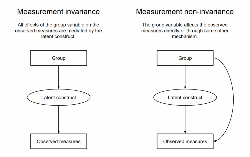
In the scenario with measurement invariance, all the group differences in the observed measure can be “explained away” by group differences in the latent construct. That also means that if we do know the group differences in the latent construct (Group → Latent construct), we essentially already know what’s happening on the item level. To figure out the precise group differences in the items, we would still additionally need the measurement model (Latent construct → Observed measures); this would for example inform us that the latent construct has only weak effects on a particular item, which in turn tells us that the group difference on that item will be smaller. But anyway, in this scenario, the group differences on the latent construct are a good summary of the group differences in the observed items and we might as well skip reporting the group differences for each single item.
That is not the case in the scenario in which there is no measurement invariance. Here as well, group differences in the latent construct will lead to group differences in the items, but there are also group differences in the items that arise through some other mechanism. Thus, the group differences in the latent construct no longer give us the full story of what is going on on the item level.
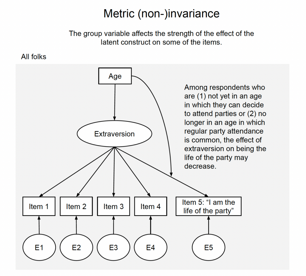
Let’s tie that back to metric invariance and our extraversion example, Fig. 4. Among very young people (who cannot yet decide on their own whether they can attend parties) or very old people (for which party attendance is no longer normative), reporting to be “the life of the party” may be less reflective of extraversion. This means that the effects of extraversion on item responses are modified by age, which could be depicted by an arrow pointing on the loading. Alternatively,[9]If you don’t want to make Richard McElreath unhappy in DAG style, you could just draw an arrow from age to the item; because everything is fully non-parametric in a DAG, all variables that jointly affect another one may interact in any conceivable way. In any case, just looking at the Age → Extraversion part wouldn’t tell us the full story about what is going on with the “variant” Item No. 5.
Probably the most intuitive examples for metric non-invariance are cases in which the effects of the factor on at least one item will vary dramatically between groups, to the point that it ceases to be a good item in one group. On Bluesky, Ed Hagen shared a wonderful example: an intelligence test item in which kids are supposed to identify what is missing from a picture. The picture shows two ice skaters, and on one of the ice skates a blade is missing. That’s easy enough to spot if you know anything about ice skating. However, the test was used to measure intelligence in South African children. That’s probably not the best item to measure intelligence in a context in which ice skating likely is a much more niche hobby than in North America.
Level 3, scalar invariance: In(ter)ception
Scalar invariance means that for each item, the intercept is the same. The statistical way to put this is a bit opaque; it means that when the observed scores are regressed on each factor, the intercepts are equal across groups. This means that group differences in the item responses are fully accounted for by group differences in the latent construct.
From a causal perspective, scalar invariance is violated if the group variable affects the item scores through some mechanism that is not the latent construct. Now, above we already said that this is the case when metric invariance is violated, but the causal story behind the violation is a slightly different one. Above, the group variable affected the magnitude of the effect of the construct on the item (which led to differences in the loadings). One could also say that when metric invariance is violated, there’s an interaction effect that we don’t want (group variable x construct → items). Here, considering violations of scalar invariance, the group variable “directly” affects the item responses. One could also say that there is a main effect that we don’t want (group variable → items).[10]If you’re more of a dag person: In a proper DAG, violations of metric invariance and violations of scalar invariance would look the same because all variables that jointly affect another one are allowed to interact by default without any need for arrows on arrows.
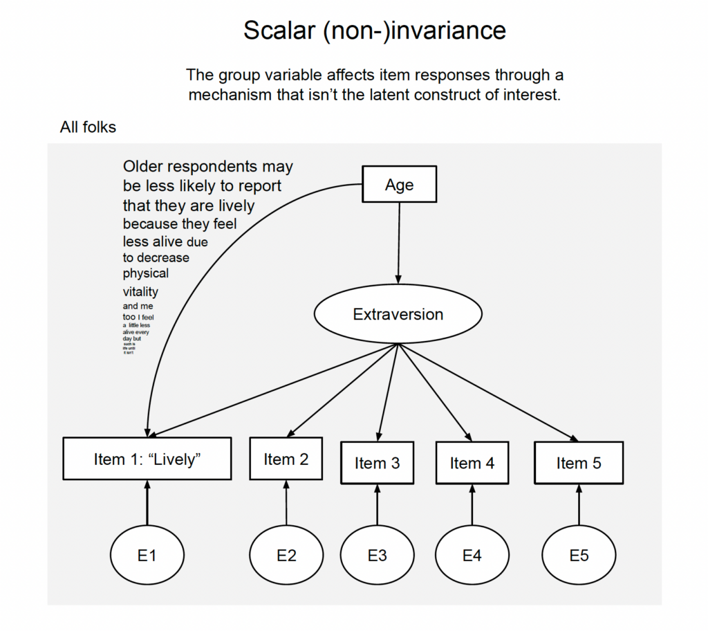
For example (Fig. 5), regardless of whatever effect age has on extraversion, age may additionally make respondents feel less vital and thus less likely to report that “lively” describes them well. In such a scenario, there will be age differences in the variant item that are not explained by age differences in extraversion.
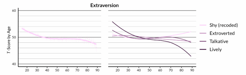
That’s what we found in an analysis of Australian data: “Lively” goes down quite a bit with age (Fig. 6), and this isn’t just age differences in extraversion (Seifert et al., 2023). There is something else that makes people feel less lively as they age, and it kicks in early. Now that I think about it, maybe this depressing finding isn’t the best way to sell our paper.
Anyway, we were interested in age effects on self-reported personality and analyzed longitudinal panel data from Australia, Germany and the Netherlands. In general, metric invariance actually seemed unproblematic in those data; the data were mostly compatible with a model in which the effects of the personality traits on the item responses are the same for people at different ages (equal loadings). But things looked much worse for scalar invariance.[11]To test measurement invariance over age, without artificially splitting people into age groups, we applied local structural equation modeling (LSEM). Think of it as multigroup SEM across individual years of age, but estimated in a manner that parameters change smoothly with age rather than bouncing around. This, in turn, opens up the possibility that for individual items, the age effects look quite different than for the factor. So we also looked at the age trajectories of the individual items to see which items diverge. That may seem like an anticlimactic “solution” to measurement invariance; it doesn’t involve any sophisticated modeling. But from my perspective, it’s true to the idea that if there is measurement invariance, that means that the latent variable does not tell the whole story that is to be told on the item level. So, why not tell the story on the item level? That may not always be an option in small data sets, but for us it was.
What other ways forward could there be?
Regarding liveliness—if we want to insist that all age effects on such items must be mediated through latent constructs—one solution would be to consider that extraversion may consist of multiple subfactors with different age trajectories. The Big Five Inventory 2 (BFI-2) splits up extraversion into three dimensions, sociability, assertiveness, and energy level. “Lively” belongs to energy level which likely shows the most pronounced age decline; “Shy”, “Extroverted”, and “Talkative” likely belong to sociability which we would expect to show less pronounced age effects. In such a manner, measurement invariance could be restored once the set of included items had been expanded, and we could once again start working with the latent variable.
Another way to more immediately restore measurement invariance would be to kick out the offending item. That may of course shift the meaning of the latent factor away from what was originally intended and may reduce comparability across studies, but I’m sure this could sometimes be a sensible solution–if implemented transparently. Readers should be fully aware of which items end up in the model that produces the final results, but that of course holds for all latent variable models. (#AlwaysLookAtTheItems)
Another approach aims at establishing “partial invariance”, which relies on some items being assumed to be invariant (thus providing an anchor for comparisons), while others are allowed to “function differentially.” And there is a lot more stuff being discussed in the psychological methods community–see for example Robitzsch and Lüdtke (2022) who argue that measurement invariance is not a prerequisite for meaningful and valid group comparisons.
I feel like in psychology, there’s a tendency to only consider the measurement model itself as if it were some free-floating thing, and then go on and tinker with it. But, for example, there is no reason to insist that all effects on personality items are mediated through invariant personality constructs. So, alternatively, we could try to model additional pathways from age to lively; maybe the “invariant intercepts” can partly be explained by adding some measure of physical health that provides an alternative pathway from age to liveliness. This step requires some degree of domain knowledge, which is always the case when it comes to causality.
Level 4, residual invariance: All that’s left
Residual invariance means that for each item, the residual variance—the variance of the ominous E pointing into the items—is the same. We can again phrase this statistically: if we regressed the item scores on the factor, then the variance of the remaining residual would be the same in the groups (i.e., there would be homoscedasticity). If this is violated, multiple causal stories could go on here. For example, with increasing age, the effect of the latent construct on the item responses could remain the same on average but become more uncertain, leading to more variability in the residuals at higher ages. But it could also be possible that, with increasing age, the effects of some variables unrelated to the construct of interest become more pronounced, or maybe new factors start to affect the item response with increasing age and thus induce additional residual variance. The thing about the residual is that it captures everything that’s not explained in the model, and explaining changes in the amount of unexplained things seems a bit futile. Residual invariance is often not tested because it’s not necessary for latent mean comparisons. It’s a bit of an anticlimactic level to end on.
Not all that’s invariant is measurement invariance
Sometimes, people will bring up measurement invariance when they have a particular mechanism in mind that may render item responses incomparable between groups. To figure out what will be flagged as a violation of measurement invariance, it helps to draw the causal graph one has in mind.
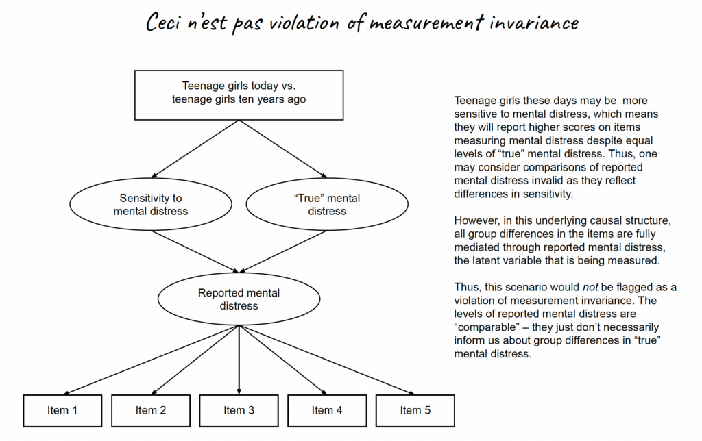
For example, consider a hypothetical scenario in which teenage girls today report higher levels of mental distress than teenage girls ten years ago. Somebody may raise the issue that nowadays mental health is discussed a lot more, and so teenage girls today may simply be more sensitive to symptoms, giving higher responses to items asking about mental distress even when the underlying level of mental distress is the same. That would render item responses incomparable in a certain sense, and one might thus suspect that this would be revealed once we test for measurement invariance.
But consider the graph in Fig. 7, in which “girls these days” are indeed reporting different levels of mental distress at least partly because of differences in sensitivity. But this actually does not violate measurement invariance (as tested in tests of measurement invariance), because all group differences are still mediated by the latent variable that is being modeled, reported mental distress: Teenage girls today may have different levels of true mental distress which leads to reported mental distress which leads to higher item responses (the “good” path that we would want to target); teenage girls today may have different levels of sensitivity to mental distress which leads to reported mental distress which leads to higher item responses (the “bad” path that some would consider spurious).
So, this is a measurement concern that would not result in a statistically detectable violation of measurement invariance. You are measuring “the same thing” (reported mental distress), but it is not exactly the thing you are trying to get at (“true” mental distress). The flip side of this is that it may look like your measure is invariant, but that doesn’t mean that the intended inferences are automatically valid.
Going a step further, measurement invariance may also occur…without any meaningful measurement. John Protzko has a study in which respondents filled out either the search for meaning in life [sub]scale, or the very same scale, but any mention of meaning or purpose was replaced with the (meaningless) term “gavagai.” Taking the questionnaire version as group variable, search for meaning in life and search for meaning in gavagai seemed to be invariant (equal form, equal loadings and equal intercepts couldn’t be rejected). He concludes that measurement invariance is at best a necessary condition for showing evidence that one is measuring the same thing in different populations; given that it may hold even when nothing meaningful is being measured in one group. I find this quite comforting: we humans may sometimes be unable to tell whether a scale measures anything at all, but at least measurement invariance doesn’t know better either. So I concur with John’s conclusion to the extent that I am willing to simply copy it to conclude this content.[12]Crémieux kindly reached out to me to inform me that actually, John’s analysis may simply be missing violations of measurement invariance that are clearly there when the data are analyzed correctly. Jordan Lasker makes this point in a preprint and provides a re-analysis. And here I thought I had found a nice way to wrap things up with an empirical finding…
Too long; didn’t read
Statistically, when we test measurement invariance, we test whether certain parameters are equal across groups within factor models. From a causal perspective, measurement invariance means that all effects of the group variable on the observed measures are mediated by the latent factor. The whole reasoning is conditional on the assumption that the latent variable model holds to begin with.
Too short; want to read more
Philipp Sterner, Florian Pargent, Dominik Deffner, and David Goretzko just dropped a cool preprint titled “A Causal Framework for the Comparability of Latent Variables.” Many of our points overlap, but they use a different framing and make use of selection nodes as they are building on a framework for generalizability. While the serious article format doesn’t allow for many memes (booh!), they make up for it by providing a lot more technical detail and examples.
Many thanks to John Protzko who provided helpful feedback that led to some additions to this blog post, and to Ingo Seifert who took a critical look as well. As always, all errors aren’t theirs but my co-bloggers’.
Footnotes
| ↑1 | A possible exception to this may be the literature on intelligence, in which measurement invariance is a relevant topic of substantive debate. |
|---|---|
| ↑2 | John Protzko told me he received pushback for saying that people say measurement invariance implies that the measure measures the same thing in different groups. So, in his preprint on measurement invariance, he now reviews the evidence that measurement invariance is commonly interpreted this way–which it is. |
| ↑3 | A little bit worse may be okay. Always check with your local statistician or the literature if you have any concerns about debates about the appropriate cut-offs for measurement invariance testing. |
| ↑4 | More technically, the data that are being explained in structural equation models are usually the elements of the variance-covariance matrix (a matrix that for each item contains its variance and its covariance with all other items; think correlation matrix but in unstandardized). Thus, SEM results can often be fully reproduced from the variance-covariance matrix alone. Sometimes, the mean structure is also modeled (e.g., when testing scalar invariance, see later section). |
| ↑5 | Here I am subscribing to a realist interpretation of factor models, in which the arrows are arrows and not a shorthand for “an association but somehow also directed.” The realist stance is forwarded in older writings by Borsboom, Mellenbergh and van Heerden (2003, 2004). A lot of researchers are probably more comfortable subscribing to a pragmatist interpretation in which a factor model is just a good way of summarizing a large number of items. I am not sure such an interpretation is 100% consistent. First of all, when calculating a factor score, items with higher loadings will have a bigger impact. Statistically speaking, those will be the items that have higher correlations with other variables. But why would we want to give higher weight to those items when the goal is to simply summarize the variables? Giving equal weights to the items (aka, just taking the average) seems more justifiable if we are completely agnostic to what caused the data (and thus also about how error may have affected values). Second, once we try to do anything else with those latent variables, inferences can end up badly biased if the true data generating mechanism was a different one (Rhemtulla et al., 2020). Unless somebody convinces me otherwise (come at me pragmabro), I think the pragmatist interpretation is mostly a cope to avoid facing that much of empirical psychology rests on very strong assumptions. That puts “I’m just using this factor model for pragmatic reasons” into the same category as “oh no I do not want to make causal claims I am just trying to do prediction” (see footnote 12) and “non-causal mediation analysis” (which isn’t a thing; mediation is statistically indistinguishable from confounding–the difference lies in causal assumptions). |
| ↑6 | And then shortly afterwards I stumbled across it again in Paulewicz and Blaut’s paper on the general causal cumulative model of ordinal response. Baader-Meinhof much |
| ↑7 | More generally speaking (and still keeping things casual), measurement invariance implies that all group differences in the items “go through” the latent construct. So, measurement invariance would also be violated if there is a common cause that confounds the group variable with the items. In such a scenario, the measure would be non-invariant, but it is a type of non-invariance that can be “explained away” if we additionally observe and model the common cause (which would allow us to arrive at unbiased conclusions about group differences in the latent construct, despite non-invariance). After posting the blog post, Borysław Paulewicz kindly reached out to me and patiently explained what a complete, causal definition of measurement (non-)invariance has to look like. You can find it on page 14 of his manuscript on the general causal cumulative model of ordinal response. It says that a response R (in our case, the observed items) is a biased measure of the latent construct T with respect to some manifest variable V (in our case, the group variable) if there exists an active causal path (one without a collider) between the response R and the manifest variable V such that the latent construct T is not a node on this path. |
| ↑8 | I have collapsed the multiple items into a single “observed measures” nodes because that looks more elegant (in DAGs, a single node for multi-dimensional variables is fair game), and also because we can think about measurement (in)variance in scenarios in which there is only a single item or outcome. We wouldn’t be able to test it with the standard procedures, but that doesn’t mean that it couldn’t be a potential concern if we have some indication that the single item could function differently in groups. |
| ↑9 | If you don’t want to make Richard McElreath unhappy |
| ↑10 | If you’re more of a dag person: In a proper DAG, violations of metric invariance and violations of scalar invariance would look the same because all variables that jointly affect another one are allowed to interact by default without any need for arrows on arrows. |
| ↑11 | To test measurement invariance over age, without artificially splitting people into age groups, we applied local structural equation modeling (LSEM). Think of it as multigroup SEM across individual years of age, but estimated in a manner that parameters change smoothly with age rather than bouncing around. |
| ↑12 | Crémieux kindly reached out to me to inform me that actually, John’s analysis may simply be missing violations of measurement invariance that are clearly there when the data are analyzed correctly. Jordan Lasker makes this point in a preprint and provides a re-analysis. And here I thought I had found a nice way to wrap things up with an empirical finding… |