[Update: After this post had been published, Uli Schimmack and I had a quick chat and Uli was very surprised to learn that I hadn’t read his 2012 Psychological Methods paper on the topic. He has now published a blog post with an abridged version of that article, including some new comments from his 2018 perspective. Check out Why most Multiple-Study Articles are False: An Introduction to the Magic Index!]
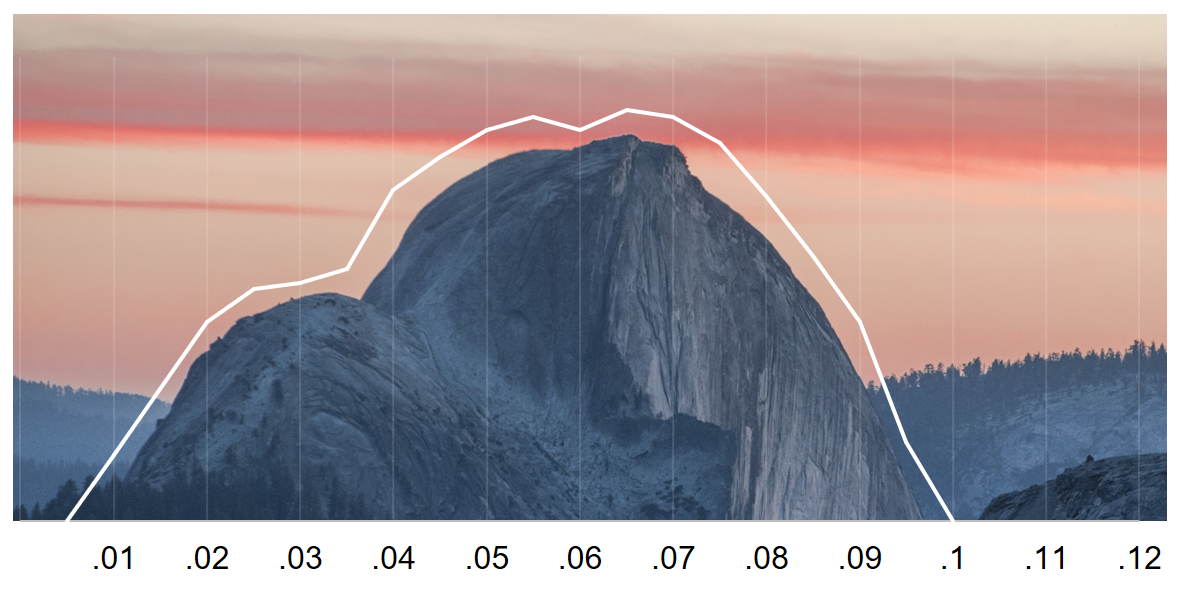
Study 1: In line with our hypothesis, … p = .03.
Study 2: As expected, … p = .02.
Study 3: Replicating Study 2, … p = .06.
Study 4: …qualified by the predicted interaction, … p = .01.
Study 5: Again, … p = .01.
Welcome to the uncanny[1]Nick Brown has (correctly) pointed out that we were probably thinking of the German word unheimlich which means, among other things, eerie, uncanny, scary, eerily, sinister, creepy, and weird—in other words, it really doesn’t translate well. Fun fact, the term uncanny valley can be traced back to Freud’s “The Uncanny” (“Das Unheimlich”). p-mountains, one of the most scenic accumulations of p-values between .01 and .10 in the world! Over the course of the last years, many psychologists have learned that such a distribution of p-values is troubling (see e.g. blog posts by Simine Vazire and Daniël Lakens) and statistical tools have been developed to analyze what these distributions can tell us about the underlying evidence (Uli Schimmack’s TIVA, p-curve by Simonsohn, Nelson and Simmons p-curve)—as it turns out, quite frequently, the answer is not good news.
However, the uncanny p-mountains can still be seen in journal articles published in 2018.[2]In fact, this blog post exists because somebody forwarded me the table of content of the current issue of a psychological journal, of which the first article I opened had uncanny p-values. And this is probably no surprise given that (1) our intuitions about something as unintuitive as frequentist statistics are often wrong and (2) many researchers have been socialized in an environment in which such p-values were considered perfectly normal, if not a sign of excellent experimental skills.[3]Such as the extraordinary ability of quickly spotting all p-values below .05 in a massive correlation matrix—a masterful art that might go extinct within a few academic generations. Or so one would hope. So let’s keep talking about it!
What’s so uncanny about p-mountains between .01 and .10?[4]One can also define a narrower mountain-range of p-values between .01 and .05. However, I have noticed that quite a few (newer) journal articles also report “marginally significant” p-values between .05 and .10 and then either (1) ignore the fact that the p-values missed the conventional threshold or (2) end the paper with a mini-meta, in which the marginally significant p-values are smoothed. However, a naive mini-meta is problematic and cannot be interpreted if the p-values misbehave—GIGO strikes again. In short, they indicate that the p-values misbehave—it is not a pattern we should encounter “in the wild”, at least not very frequently. And they should worry us because they tell us that something is off about the statistical evidence—the centerpiece of every quantitative empirical journal article.[5]Of course, sound statistical evidence is not sufficient to render any specific empirical claim valid. After all, there are other things that can go wrong, like the design of the study. However, sound statistical evidence is necessary for any empirical claim to be taken seriously.[6]Sufficient vs necessary: If A is sufficient for B, that means whenever A is true, then B is also true. For example, eating a tray of cookies is sufficient for me to feel full. Whenever I eat a tray of cookies, I will feel full. However, I might also feel full without having eaten a tray of cookies–for example, if I ate a whole cheesecake instead. If A is necessary for B, that means you cannot have B without A. For example, it is necessary for me to get out of bed to be able to run a marathon. If I stay in bed, I can’t run a marathon. However, it doesn’t mean that whenever I get out of bed, I will automatically be able to run a marathon. For example, I might get out of bed, but then eat a whole tray of cookies and a cheesecake on top, so I won’t be able to run a marathon.
The uncanny p-mountains are unlikely if the null hypothesis is true
First of all, we would not expect to see the uncanny p-mountains if we ran a series of studies and tested for an effect that was actually not there. If the null hypothesis (either no effect, or an effect in the opposite direction—we are assuming that all observed effects point into the “theory-conform” direction) was true, then there is a 3% chance that we observe p ≤ .03—a rare event, but certainly not extraordinarily rare. It’s like rolling two fair, six-sided dice and getting double sixes. But now comes the second study, p = .02. Observing p ≤ .02 in isolation again has a probability of 2% if the null is true, which is again not extraordinary. However, the joint probability of running two experiments in a row and observing p = .03 and p = .02 is lower. If you use Fisher’s method for combining independent p-values, you get p = .005, or 0.5%.[7]Many thanks to both Roger Giner-Sorolla and Aurélien Allard for making me aware of Fisher’s method for the combination of independent p-values! That is indeed rather unlikely, like rolling triple sixes.[8]It’s also comparable to the probability of a Shadow Brute dropping a Prismatic Shard—and if you’ve played Stardew Valley, you know these Prismatic Shards are freaking hard to get. I managed to get two because I’m a filthy grinder.
And now we can just keep applying the rule to find out that the combination of p-values as low as the ones shown at the beginning of this post are extremely unlikely if the null hypothesis is true (.00003). Likewise, if we apply the conventional alpha-threshold, 5 p-values that pass p < .05 are extremely unlikely if the null is true (.05^5 = .0000003125). And even if we apply more generous thresholds and include p-values that are “approaching” significance (whatever that is supposed to mean; here is a list of 508 additional creative ways to label non-significant p-values), it’s still an unlikely event (.10^5 = .00001).
Good news: The data are not compatible with the null hypothesis! However, here comes the bad news: They’re not compatible with the alternative hypothesis either.
The uncanny p-mountains are unlikely if the alternative hypothesis is true and statistical power is decent
How likely is a p-value, given that the null is wrong and there is an effect? Thankfully, Daniël Lakens (see blog post mentioned above) and JP de Ruiter[9]JP derived the formulas from scratch as an exercise, so it would probably be most accurate to say that he did the math. There is also an article from 1997 doing the math in Biometrics and I’m sure multiple people have done it before. have done the math and Kristoffer Magnusson has turned it into an extremely nifty interactive visualization which you can find here. For example, let’s assume that you are comparing two groups, the true difference between the two groups is d = .4, and following ye olde stats textbook, you collect N = 99 per group to achieve a statistical power of 80% (using the conventional .05 cut-off). Now, not very surprisingly, you have an 80% chance to get a p-value between 0 and .05. However, zooming in on the p-values between 0 and .05, it is actually three times more likely to get a p-value between 0 and .01 (about 60%) than to get a p-value between .01 and .05. Even if you apply a more liberal criterion, a p-value between 0 and .01 is still twice as likely as a p-value between .01 and .10! The chances of running five “adequately” powered studies and always landing in that sweet .01 to .10 range are again rather small, or 0.2%. This should happen once in a blue moon, but probably not twice in one journal issue, and certainly not routinely across whole fields of research. Notice that the logic here is a slightly different one: Above, we observed that the central tendency of the point estimates were unlikely under the null hypothesis that the real effect is zero or pointing into the opposite direction. Here, we observe that the lack of variability in p-values is unlikely under an alternative hypothesis (i.e., we reject the null hypothesis that their variability is normal).
If the null hypothesis is false, the shape of p-values above .01 should not form an uncanny mountain, but a canny valley.
So far, we have been assuming decent power. However, decently powered studies are the exception, not the norm. So maybe underpowered studies can account for the pattern?
Low power is not a sufficient explanation for the uncanny p-mountains
Let’s assume we instead had a power of 50% to detect an effect with p < .05. That means chances to find the effect given its existence are like the flip of a coin. At this level of power, p-values between 0 and .01 get rarer (but you can still expect them around 27% of the time) and are only slightly more likely than p-values between .01 and .05 (~23%), but less likely than p-values between .01 and .10. In other words, low power results in a relative increase of p-values above .01.
But here comes the crux: At 50% power, half of your studies will not reach the significance threshold of p < .05. If you run five studies with 50% power in a row, it is unlikely that all of them turn out statistically insignificant (.50^5 = .0315, or 3.15%). You get somewhat “better chances” if you use the threshold of p < .10, though it’s still not super likely (around 9%).[10]For reference, that is about the chance that among 9 people, at least two share the same birthday (same day and same month).
But it might certainly happen in a few studies! However, of these (more or less) significant p-values, many will again lie between 0 and .01. The chances of running five underpowered studies in a row and getting p-values between .01 and .10 are about .006, or 0.6%. And again, that is rather unlikely, though of course not impossible.

The uncanny p-mountains cannot be explained by “exact power”
One argument that has been raised is that experts are able to power their study “just right” to get the desired significant effect (p < .05) without wasting excess resources, a.k.a. valuable research participants (p not much smaller than .05, following the Goldilocks principle “just the right amount of significance”). Let’s assume the notion of expertise was right in principle. An expert might be better at detecting an effect at a given sample size because s/he expertly designed the study in a way that maximizes the effect size (better manipulation, better outcome measure) or tames random factors affecting the study (which has, in fact, the same result: a larger effect size).
In other words, let’s assume that experts can increase the signal or decrease the noise. What would that mean? It would mean that all else being equal, they would have higher statistical power and thus more p-values below .01 relative to p-values between .01 and .05 than the average non-expert scientist. So that can’t be the explanation.
What if they had higher power thanks to expertise, but then strategically decreased sample size to save valuable resources? Well, that would either result in the same power as the average non-expert scientist, or lower power. Neither of the two could explain the pattern of p-values.
Maybe there’s something else that experts do that influences p-values without going through the “normal” channels of statistical power? Well, it wouldn’t be accommodated for in the prevalent statistical models, and frankly, everything I can come up with would defy the laws of stochasticity. However, if you can come up with an explanation that is not paranormal, let us mortals know.
So, who raised the uncanny p-mountains?
First, of course, even an uncommon pattern will sometimes arise by chance. It is possible that some researchers get extremely lucky with underpowered studies (but even then they should probably be informed that their research is, well, underpowered). It is still technically possible that somebody gets repeatedly extremely lucky, but the probability quickly approaches 0.
So let’s talk QRPs: Questionable Research Practices. It is rather easy to get accumulations of p-values just below .05 by running “flexible” analyses until something reaches the conventional cut-off (Simmons, Nelson, & Simonsohn, 2011). And remember the five underpowered studies in a row that all yielded p < .05? Well, if the authors ran a lot more studies but did not disclose those that failed to support their hypothesis, the extremely rare event turns into something much more probable.[11]In Stardew Valley terms, void essence. What on earth am I supposed to do with all of that void essence?
This might make some people feel uncomfortable: How could we deduce from a pattern that is unlikely but still possible to have arisen by mere chance that somebody did something wrong?
It might help to keep in mind that many practices that are filed under QRP are pretty damn common. For example, a quick glance at either John, Loewenstein, and Prelec (2012) or Agnoli, Wicherts, Veldkamp, Albiero and Cubelli (2017) reveals that many practices, such as failing to report all dependent measures or selective reporting of studies that “work” are very common. There are a tons of degrees of freedom in planning, running, analyzing and reporting studies (nicely listed in Wicherts et al., 2016), some of which might even be considered best practices by some (e.g., measuring the dependent variable in several alternative ways, trying out different ways to score the chosen primary dependent variable).
If these degrees of freedom are dealt with carelessly, we get questionable research practices. Researchers need not even be aware of the questionable nature of what they are doing—in many cases, model modifications might make a lot of sense after the fact.[12]Simonsohn, Simmons & Nelson talk about defensible yet arbitrary data analytic decisions. And as Gelman & Loken stress in their “Garden of Forking Paths”, this can all happen without any conscious fishing expeditions. For example, isn’t it obvious that X should be controlled for? Of course, outcome Y didn’t work, well thank Glob we also included outcome Z! The problem is that, usually, the motivation to make these modifications is greater when initial analysis fails to confirm cherished hypotheses. So no single researcher necessarily did something s/he considered wrong, but we end up with a literature filled with implausible p-value patterns. And that is tragic for everybody involved because it means that often, we will not be able to judge from a study or a body of studies whether there is substantial evidence to support a conclusion.[13]If you want a particularly impressive example, take a look at this website on quantification strategies for the Competitive Reaction Time Task (CRTT). There are more ways to analyze this measure than publications including it (which means that some publications include multiple quantification strategies). That almost guarantees that researchers will always find something where they can claim p < .05, but it also means that the literature becomes practically uninformative. That does not mean that we know for sure that the claimed effects do not exist—it means that the existing data cannot tell us.
Erosion is a slow and steady process
Understanding what distributions of p-values look like in different conditions—and making sure that our students also have an idea of what healthy p-values look like—might be the first step to get rid of the inflation of p-values between .01 and .05/.10. More awareness would also enable researchers to catch themselves at fooling themselves (or, as Simine Vazire puts it, it would help them be their own a**holes). Fooling oneself is horribly easy,[14]There should be a drinking game in which everybody has to drink when somebody cites Feynman in the context of the replication crisis. Just make sure that you use a drink with < 5% or maybe even < .05% alcohol. which is why it might in many cases be necessary to preregister analyses: Afterwards, you will be able to tell whether that .03 really just occurred by chance, or whether you convinced yourself that out of all possible analyses, that one was the most plausible. Of course, this is assuming that researchers are motivated to find the truth. Personally, I believe that this motivation is the norm, but others might disagree. And sure, maybe God loves the .011 just as much as the .009—but what does he know, he doesn’t even have a paper in JPSP!

Of course, motivation is also partly shaped by incentives. If I can publish an article with ten p-values at the brink of .05, why would I even start to think about whether there is something wrong with the way that I analyze data? Editors and reviewers can make a huge difference by pointing out implausible p-value patterns. So the next time you review a manuscript with uncanny p-mountains, don’t just enjoy the scenery: Ask some critical questions because that’s the purpose of peer-review.
But isn’t it wrong that single researchers, who might have just gotten (un)lucky, are under suspicion for the vices of the field? Well, yes, but this is part of the whole tragedy: Rampant abuse of p-values has made it impossible to discern the (rare) legit occurrence of multiple p-values above .01.
Given that researchers now know what signal the mountain sends, they can choose to add a final preregistered replication to make it a convincing set. Change has to start somewhere!
Footnotes
| ↑1 | Nick Brown has (correctly) pointed out that we were probably thinking of the German word unheimlich which means, among other things, eerie, uncanny, scary, eerily, sinister, creepy, and weird—in other words, it really doesn’t translate well. Fun fact, the term uncanny valley can be traced back to Freud’s “The Uncanny” (“Das Unheimlich”). |
|---|---|
| ↑2 | In fact, this blog post exists because somebody forwarded me the table of content of the current issue of a psychological journal, of which the first article I opened had uncanny p-values. |
| ↑3 | Such as the extraordinary ability of quickly spotting all p-values below .05 in a massive correlation matrix—a masterful art that might go extinct within a few academic generations. Or so one would hope. |
| ↑4 | One can also define a narrower mountain-range of p-values between .01 and .05. However, I have noticed that quite a few (newer) journal articles also report “marginally significant” p-values between .05 and .10 and then either (1) ignore the fact that the p-values missed the conventional threshold or (2) end the paper with a mini-meta, in which the marginally significant p-values are smoothed. However, a naive mini-meta is problematic and cannot be interpreted if the p-values misbehave—GIGO strikes again. |
| ↑5 | Of course, sound statistical evidence is not sufficient to render any specific empirical claim valid. After all, there are other things that can go wrong, like the design of the study. However, sound statistical evidence is necessary for any empirical claim to be taken seriously. |
| ↑6 | Sufficient vs necessary: If A is sufficient for B, that means whenever A is true, then B is also true. For example, eating a tray of cookies is sufficient for me to feel full. Whenever I eat a tray of cookies, I will feel full. However, I might also feel full without having eaten a tray of cookies–for example, if I ate a whole cheesecake instead. If A is necessary for B, that means you cannot have B without A. For example, it is necessary for me to get out of bed to be able to run a marathon. If I stay in bed, I can’t run a marathon. However, it doesn’t mean that whenever I get out of bed, I will automatically be able to run a marathon. For example, I might get out of bed, but then eat a whole tray of cookies and a cheesecake on top, so I won’t be able to run a marathon. |
| ↑7 | Many thanks to both Roger Giner-Sorolla and Aurélien Allard for making me aware of Fisher’s method for the combination of independent p-values! |
| ↑8 | It’s also comparable to the probability of a Shadow Brute dropping a Prismatic Shard—and if you’ve played Stardew Valley, you know these Prismatic Shards are freaking hard to get. I managed to get two because I’m a filthy grinder. |
| ↑9 | JP derived the formulas from scratch as an exercise, so it would probably be most accurate to say that he did the math. There is also an article from 1997 doing the math in Biometrics and I’m sure multiple people have done it before. |
| ↑10 | For reference, that is about the chance that among 9 people, at least two share the same birthday (same day and same month). |
| ↑11 | In Stardew Valley terms, void essence. What on earth am I supposed to do with all of that void essence? |
| ↑12 | Simonsohn, Simmons & Nelson talk about defensible yet arbitrary data analytic decisions. And as Gelman & Loken stress in their “Garden of Forking Paths”, this can all happen without any conscious fishing expeditions. |
| ↑13 | If you want a particularly impressive example, take a look at this website on quantification strategies for the Competitive Reaction Time Task (CRTT). There are more ways to analyze this measure than publications including it (which means that some publications include multiple quantification strategies). That almost guarantees that researchers will always find something where they can claim p < .05, but it also means that the literature becomes practically uninformative. That does not mean that we know for sure that the claimed effects do not exist—it means that the existing data cannot tell us. |
| ↑14 | There should be a drinking game in which everybody has to drink when somebody cites Feynman in the context of the replication crisis. Just make sure that you use a drink with < 5% or maybe even < .05% alcohol. |
As usual, great post and great jokes! I had always assumed that God must have more impressive credentials. One small comment about a small mistake (or simplification?): you can’t combine p-values by simply multiplying them. You have to use special techniques, like for instance Fisher’s combined probability test (a nice intro can be found here: https://www.ncbi.nlm.nih.gov/pubmed/16135132). You can see this by taking a few p-values perfectly compatible with the null (let’s say 0.8, 0.5, 0.2, 0.1); if you multiply them, you get a value of .008, which doesn’t represent the fact that it’s a typical distribution of p-values (if you use Fisher’s exact test, the “real” p-value is the unimpressive .29). Using Fisher’s test, a combined p-value of .02 and .03 gives a p-value of .005; that’s still unlikely, but ten times more likely than it would be if you just multiplied the values.
Thanks for pointing that out, I just fixed it!
Hi, thanks for this!
I have one question, a bit naive! In the post, you refer to studies, which I would assume would refer to a series of independent experiments. What about observing the uncanny mountain in a series of “sensitivity” “robustness” checks of the kind economists usually run? Thanks!
Not naive at all, that’s actually an important point. If the p-values come from different robustness checks of the same effect within the same sample, they’re no longer independent, and it gets more likely that they’re close to each other.
For example, if you had two different outcome variables measuring the same underlying variable and detected some weak signal on one of them, it’s quite possible that the other measure also picks up a weak signal. In such a scenario, you’d have to correct for the correlation between the outcomes. However, I don’t know how you’d have to adjust in case the robustness checks include completely different model classes or inclusion of other variables. I’m not aware of any papers discussing selective reporting of robustness checks and its statistical “signature”, but that’s probably just because I mostly read psych papers, and robustness checks are not a big thing in psych (which is a problem in itself).
Somewhat related (but more on the author side of things), Simonsohn, Simmons, & Nelson suggested Specification Curve Analysis for robust inference across defensible model specifications (https://papers.ssrn.com/sol3/papers.cfm?abstract_id=2694998), so that would be one possible way to incorporate robustness checks in a more formal manner. It seems somewhat more transparent than normal “hand selected” robustness checks, but it could still be “gamed” by only including robustness checks that work.
Thanks for the paper and the insight! I remember now a post from Andrew Gelman of pooling all the robustness checks in one multilevel model, but I was never sure how to do that if you have checks on samples that are only slighty different each time or if checks include trying out different model specifications altogether
I couldn’t disagree more with footnote #14! If people engaged in such a drinking game, many people would die from alcohol poisoning…
In any case, I think you (and Simmons, Nelson, & Simonsohn) are hitting the nail on the head. Questionable research practices are not taught in classrooms, but they are routinely taught in “productive” labs. Fishing for significance is a routine practice, even though the same people who actually do it would roundly condemn the practice in undergraduate statistics classes. Hence, the uncanny mountain of which you speak…
Heh, you’re right about the drinking game! I’ll add a safety note that you should only play it with drinks with less than 5% alcohol…
As a fun side note, I actually know of one methods class (even for master’s students!) in which fishing for significance was explicitly framed as a superior strategy (“Frequent mistake of students who collect data for their theses is that they don’t collect more participants after the right trend already shows in the data”). But I really hope that’s an exception, not the rule. Students imitating the strategies of “successful” labs in which they are working is probably the biggest transmission mechanism…
Regarding the “successful labs” comment, I was thinking particularly of Smaldino’s 2016 paper on “The Natural Selection of Bad Science” (here’s the link: http://rsos.royalsocietypublishing.org/content/3/9/160384). Wish I could claim credit for that idea, but it’s simply not the case 🙂